Since early February, the financial markets have been wobbly. After the deep plunge (worst point-wise fall) of the Dow Jones in February 5, the stock markets have recovered but the market volatility has remained elevated. Many have blamed the rising inflation expectations, the more hawkish tone by the Fed and/or the economic policies (like tariffs and tax cuts) of president Trump on penalizing the nine-year old bull market. Although all these notes carry some merit, a fundamental change in the financial regime has also hit the stock markets recently.
In the late January, the quantitative tightening or the QT-program of the Federal Reserve (Fed) has got into full gear. Fed enacted the program, as the first central bank ever, already in October, but the actual decline in the asset holdings of the Fed was rather small before January. Then, just in one month, the balance sheet of the Fed fell by more than 18 billion dollars. It is naturally impossible to say whether this was the primary reason for the fall of the highly-overvalued stock market, but the timing suggests that the OT had an effect. More so, because the quantitative easing (the QE-program), supported the asset prices for several years.
QE and the banking system
The first QE, started by the Fed in 25 November 2008, aimed at purchasing the Government Sponsored Enterprise (GSE) debt and mortgage backed securities (MBS). In March 2009, the purchasing was extended to include the US Treasury debt. The aim of the Treasury purchases was to stimulate investments by lowering the long-term rates and to support consumption by boosting the asset prices. In layman’s terms, the Fed wanted artificially rise the asset prices. The Fed halted new bond purchases in October 2014. By that time its balance sheet had swollen to $4.5 trillion from around $900 billion in early 2008.
The QE-programs are usually conducted through the commercial banks. In the US, the Fed purchased securities from authorized Primary Dealers by crediting reserve balances to the accounts of banks that were associated with each dealer counterparty. Regardless of whether the ultimate seller of the security is a non-bank or a commercial bank, the reserves created through the QE were preserved in the central bank. This has some important effects on the bank lending.
First, because the commercial banks were forced to hold a higher supply of reserves, their marginal benefit decreased. This bid up the prices of various securities, leading to additional loans issued until the balance of the marginal benefits was restored. Second, because the QE:s (and low policy rates) pushed down the long term rates, many of the securities that the commercial banks can hold became closer substitutes for the reserves. This made the banks ever more likely to obtain non-liquid and riskier securities.
The QE thus altered the net interest margins, the liquidity portfolio and the duration of the assets of the commercial banks. This induced the banks to increase lending and to move their portfolio towards riskier lending activities. Thus, the QE increases the financial fragility of the banking system.
QE and financial markets
In the financial markets, the QE has two roles. First, it creates an excess liquidity environment and introduces a persistent buyer (the central bank). When the central bank purchases investment grade bonds, it increases the liquidity (money) among the private investors thus lowering the premium for illiquidity. As the demand for and thus the price of the investment grade assets are elevated, the investors look for higher yielding products such as equities. Because the central bank (the persistent buyer) provides amble liquidity for the private market participants, the market volatility decreases encouraging the investors to take more risks.
Secondly, as the amble liquidity suppresses the interest rates, it encourages the investors to increased risk taking through increasing leverage. Also, as explained above, QE increases especially the high-risk lending as well as the total lending activity of banks because it operates through the banking sector. This and the falling bond returns increase the incentive to invest in equities.
Machines, passive investment funds and active investors get accustomed to rising prices and engage in ‘buy the dip’ strategies every time the market falls. Complacency takes hold. The liquidity flow from the QE:s spreads across the globe and an ‘everything bubble’ is formed.
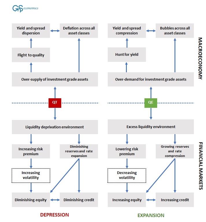
Figure 1. The causative channels of quantitative easing (QE) and quantitative tightening (QT) in the macroeconomy and in financial markets. Source: GnS Economics.
The end (QT) is nigh
There is no practical way that the central banks would be able to choose to roll-back their asset purchase programs without causing the asset markets to fall. This is because the QE -programs had such a major effect on them.
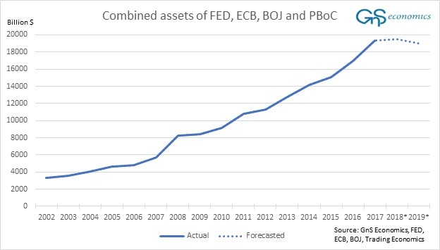
While the Fed has started its QT -program, were it is set to slash some $400 billion of assets this year and $600 billion in 2019, the European Central Bank and the Bank of Japan are still actively engaged in QE. We are thus only experimenting with the early stages of quantitative tightening. Nonetheless, the global QT should start by the end of this year, when the ECB is set to wound down its QE program (see the figure).
The effects of the Quantitative tightening are likely to remain subdued for a while. But, make no mistake, when the global pool of artificial central bank liquidity starts to withdraw, it will have dire repercussions for the asset markets. Look out below!
Download the report describing the effects of QE and QT on the real economy and on the financial markets and other reports from our Publications -page.